Autoencoder & Generative Models

Compared to discriminative models which learn the conditional distribution P(Y|X=x) directly (such as kNN, SVM, Neural Networks, etc.), generative models learn the joint distribution P(X,Y) which assumes the data is generated by the underlying distribution P(X,Y). Examples of generative models include Naive Bayes, Gaussian Mixture Models, and Bayesian Networks.

One of the interesting fields of machine learning in AI is the capability for creative activities, this can include create new images, texts, and even musics and videos. This is based on the assumption that everything around us has some statistical structure and is generated by some unknown and complex underlying process, and the goal will be using machine learning to learn this underlying structure and then sample from the statistical latent space to create new data. Generative models are for these types of tasks - learn the generating process for the training data and be able to sample from the latent space to give us new data that we might have never seen before.

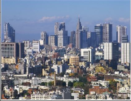
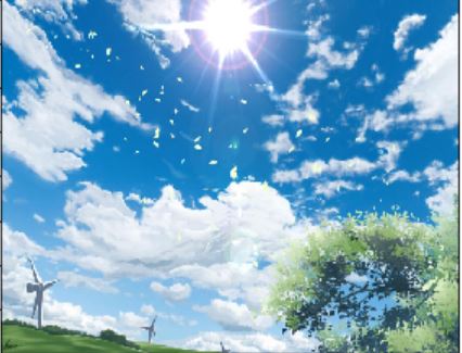
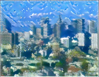
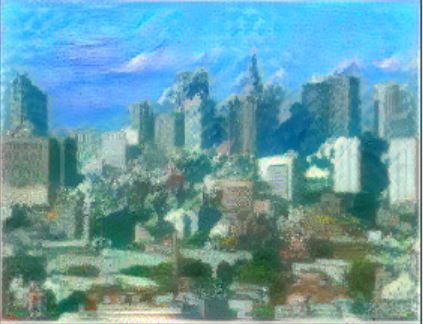
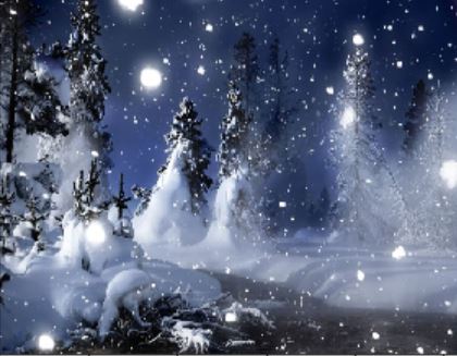
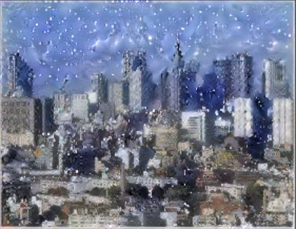
The following pictures are generated by an algorithm known as neural style transfer (as the name suggests, use deep learning algorithms to apply the style of a picture to another picture and therefore generate new pictures). As shown below, three types of styles (sky, beach, snow) from three different reference images are applied to the picture of a city view (the content image). The new generated images still have the city view content but the background (style) of the images are now being changed according to the styles of the reference images. This is done by using a simple Convolutional Neural Network (ConvNet), where the upper-level activations of the ConvNet learn the more global & abstract content of the input image and the internal correlations between activations learn the style of the reference image (as style is more local on textures, colours, etc.).

Autoencoders

Briefly speaking, autoencoders are data compression algorithms that are used to learn efficient latent representation of the data (dimension reduction) by training the model to remove the "noise" from the data. As the example shown below, an autoencoder consists of the following parts:

1. Encoder - learns the latent representation from the input data and compresses the data into a compact form (known as code or encoding)

2. Decoder - decodes the code back to a reconstructed data that ideally is similar to the input data

Examples of Autoencoders

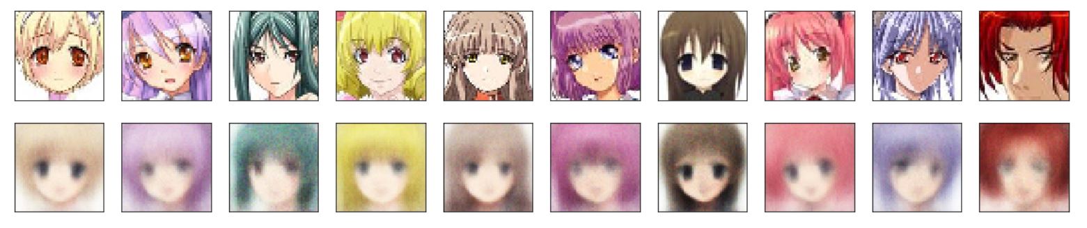
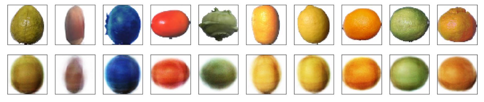
Example 1. Simple Autoencoders

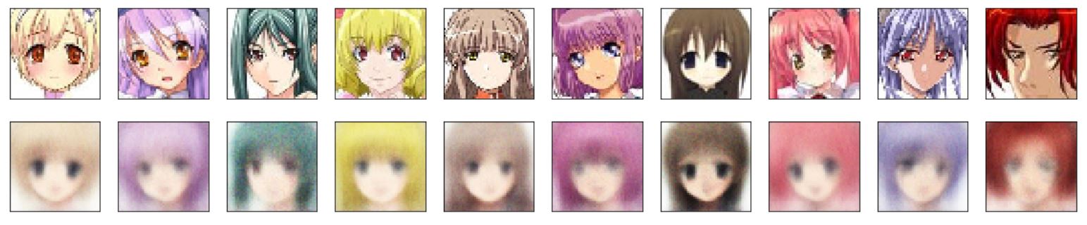
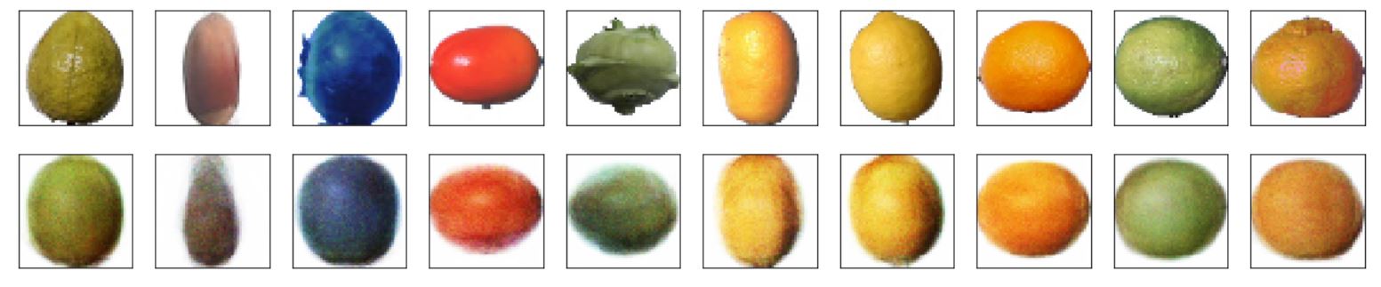
The first example uses a simple single layer neural network for both encoder and decoder. Original images are in size 50*50*3 (RGB images) which have a dimension of 7,500. The encoded latent representation has a dimension of 256 which means the compression ratio is 7500/256 = 29.3. A comparison between the original and reconstructed images are shown below. For illustrations, two different autoencoders are built on two different datasets, the first one being the Anime dataset and the second one being the Fruit dataset.

Anime dataset. Loss on the test set is 0.55 and it can be seen that the reconstructed images did not capture the original images well, but interestingly the reconstructed images have shown various styles of images in the dataset.

Fruit dataset. Loss on the test set is 0.40 and again it can be seen that the reconstructed images did not capture the original images well. Also note that the fruit images have less details than the anime images which possibly means they are easier to encode.

Remarks

A single layer autoencoder with linear activation function and squared error loss is actually nearly equivalent (same spanned subspace) to Principal Component Analysis (PCA) which projects the data into a subspace. Note that here the autoencoder is not exactly linear as the activation functions are non-linear (ReLu and Sigmoid functions).

Example 2. Deep Autoencoders

The second example uses a 3-layer neural network for both encoder and decoder. Again the encoded latent representation has a dimension of 256 which means the compression ratio is the same as the simple autoencoder. A comparison between the original and reconstructed images are shown below.

Anime dataset. Loss on the test set is still 0.55 and no improvement can be seen for the reconstructed images. Perhaps because the latent dimension is not big enough to encode the data which has very complex structures.

Fruit dataset. Loss on the test set is 0.38 and it can be seen that the reconstructed images are slightly better than that from the simple autoencoder.

Remarks

Note that deep autoencoders project the data not onto a subspace but onto a non-linear manifold which means they can learn much more complex encodings for the same encoding dimension compared to simple autoencoders and PCA. However, bottle neck on the encoding dimension can still be a big problem for encoding images with complex structures.

Example 3. Convolutional Autoencoders

The third example uses a convolutional neural network for both encoder and decoder. In this case the encoded latent representation has a dimension that is much higher than the deep and simple autoencoders which means they possess much higher entropic capacity. A comparison between the original and reconstructed images are shown below.

Anime dataset. Compared to the previous autoencoders, it can be seen that the convolutional autoencoder can encode the complex images much better, even though it still misses many of the details (especially shades of colours).

Fruit dataset. Similarly the convolutional autoencoder gives much better reconstructed images than the previous autoencoders.

Applications of Autoencoders

In practice autoencoders are not useful tools for data compression compared to algorithms such as JPEG, mainly because they are lossy (outputs will always be degraded) and the fact that they are usually very specific to the training data (data-specific and cannot be generalized to a broad range of images). However, there are many useful applications of autoencoders:

Feature extraction & Dimension reduction - autoencoders can learn more interesting features than PCA, and the extracted features can be used for visualization or as inputs for another dimension reduction algorithm such as tSNE

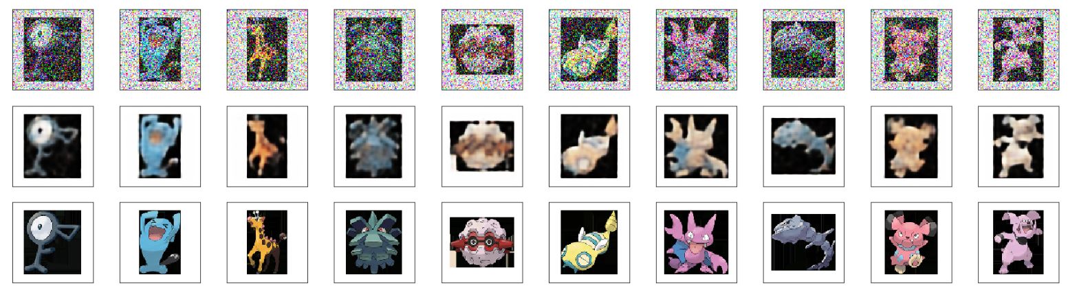
Image Denoising & Neural painting - train the autoencoder with input as clean images and target as noisy images. This technique can also be used for neural painting such as remove watermarks on photos. An example of image denoising on the anime dataset is shown below. First row being the noisy images, second being the recovered images, and the last row being the clean original images.

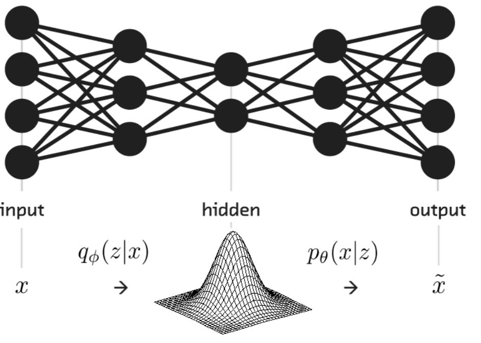
Variational Autoencoders

Compared to traditional autoencoders, variational autoencoders (VAE) are generative models - which means not only they can compress data but they can also generate new data (e.g. images) that we have never seen before. As shown in the graph below, instead of encoding the input into a fixed code, the encoder will encode the input into parameters of a statistical distribution and this allows a stochastic generation of encoded input. In other words, for the same input, the reconstructed output will be different on each single pass due to the randomness from sampling of the latent distribution.

Structured and Continuous Latent Space

The key reason that traditional autoencoders cannot generate new images is the fact that the learned latent space is discontinous, which means if the decoder never saw the encoded data before (which is very likely because there are gaps in the space) then the generated output will be unrealistic. On the other hand, by encoding the input into a probability distribution, the decoder can learn an area or cluster of points in the latent space with a wide range of variations, and the continuous latent space will not leave many gaps where the decoder has never seen before. This allows the VAE to generate variations from the training data and therefore gives us new outputs.

Reconstruction and Regularization losses

Compared to autoencoders which uses only the reconstruction loss, VAEs involve two losses:

Reconstruction loss - same as in autoencoders, this loss forces the sampled output to match the original input.

Regularization loss (KL-divergence between the latent distribution and the prior distribution) - this term helps in reducing overfitting of the model to the training data as well as helps in learning a more structured and continuous latent space. Note that the learned latent distribution is the posterior distribution.

Remarks

Choice of prior distribution - although in theory the prior distribution for the encoding can be chosen as any distribution, for example, Gaussian, uniform, mixture of Gaussians, etc, the most commonly used distribution is the standard Gaussian distribution. One of the reasons is that it can be shown that by using a standard Gaussian distribution as the prior, an analytical formula can be derived for the KL-divergence between the prior and posterior using the reparametrization trick. Note that the KL-div loss tries to force the posterior latent distribution to be the same as the standard Gaussian prior distribution.

Equilibrium between the two losses - if we consider the context that the training data can be clustered into different groups, then the reconstruction loss helps in ensuring that enough similarity of nearby encodings can be achieved by minimizing the cluster variance and segregating cluster means, while the KL-divergence loss helps in making sure that there are some overlapping between different clusters so that there are enough variations that can be made (i.e. making sure the latent space is continuous and dense so that smooth interpolation can be made). Therefore, the KL-divergence loss is a key component for training a VAE.

Disentangled variational autoencoder - Disentangled VAE is a form of VAE that tries to make sure that the hidden units in latent space are de-correlated by adding a hyperparameter to the KL-divergence loss. The goal is to create a compact latent space so that more meaningful concept vectors and feature extractions can be done.

Applications of VAEs

There are many interesting applications of VAEs, include image editing and latent space animations:

Image editing & Concept vectors - because the learned latent space supposed to be highly structured and continuous, it is possible to find concept vectors - vectors in the latent space that actually encode meaningful information of variations. For instance, by finding a "smile concept vector", we can transform a face into a "smile face".

Latent-space animations - depend on how we sample from the latent distribution, we can create a series of animations by showing an input image slowly morphing into another image through a series of intermediate transformations. Some examples are shown below.

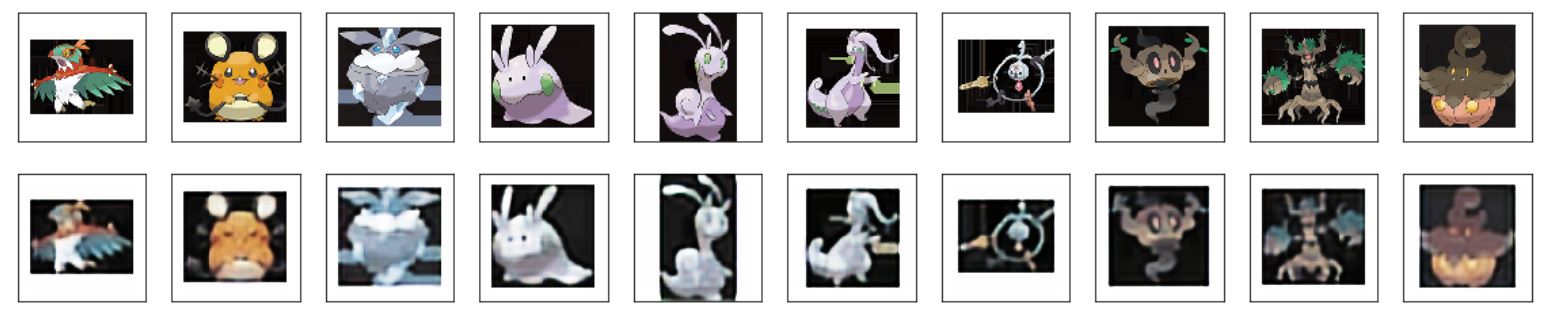
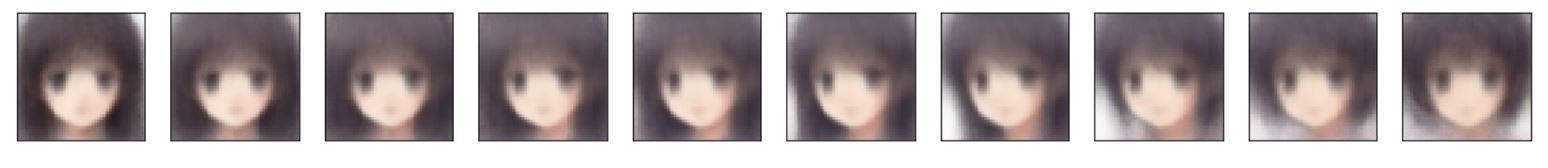
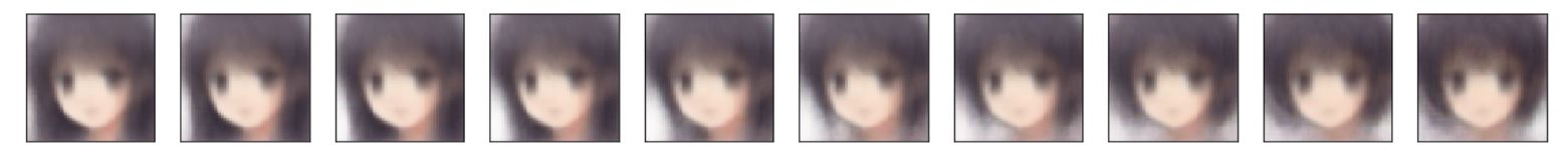
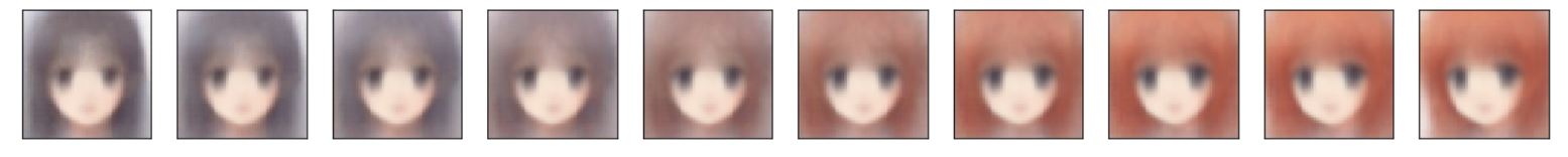
Examples of latent-spaced animations

Example 1. Anime dataset

Since the prior distribution is the standard Gaussian, the inverse CDF of standard Gaussian is used to produce values of the encodings. It can be seen that by sampling from different regions of the latent space, different samples are created and the bigger the region is, the more variations the sampled outputs can have.

Sample from 0.05-0.95 range of the standard Gaussian CDF.

Sample from 0.5-0.95 range of the standard Gaussian CDF.

Sample from 0.05-0.5 range of the standard Gaussian CDF.

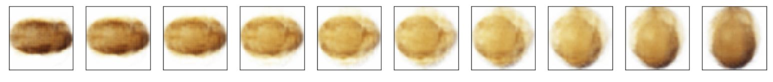
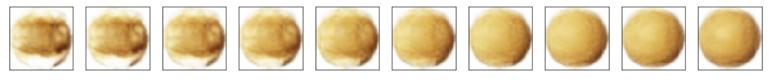
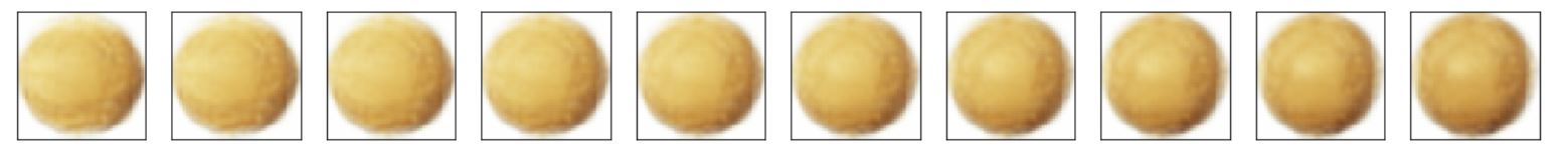
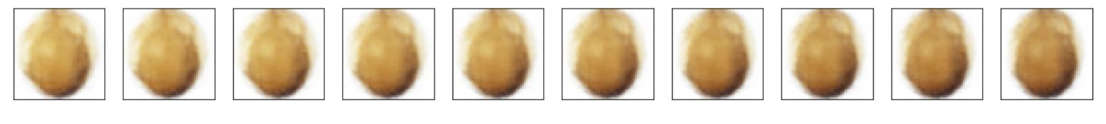
Example 2. Fruit dataset

Sample from 0.1-0.9 range of the standard Gaussian CDF.

Sample from 0.1-0.5 range of the standard Gaussian CDF.

Sample from 0.2-0.6 range of the standard Gaussian CDF.

Sample from 0.8-0.9 range of the standard Gaussian CDF.

Last updated on Apr 26, 2020