Computer vision - Classify landscape photos using CNN

This project explores how to use convolutional neural networks (CNN) on image classification problems, with only a small dataset available (few hundreds of images in this example). The actual task is as follows: given a photo of landscape, predict it is a Mountain OR Sea (binary classification). Again the goal is to develop some guidelines and insights as how to apply deep learning methods on images. Models are built using Keras.

Image data

Compared to sequence data (for example, text or time series) which can be stored in 3D tensors (sample, timestep, feature), image data is stored in 4D tensors - (sample, height width, color_depth) where the color_depth axis usually has 3 dimensions (for RBG images). For this project, each image is expressed with an (150, 150, 3) array and images are grouped with a batch size of 10 (as the total number of training sample is quite small).

The training set contains 400 photos (200 mountains and 200 seas), where both the validation and test set contain 200 photos (100 mountains and 100 seas). One of the challenges is that the "mountain" and "sea" class can contain a variety of different types of mountains and seas, for example, mountains can include rocky mountain, snow mountain, etc and seas usually contain waves, beaches, etc. In addition, the images can be taken from various sources so there are lots of distortions in the photos (for example, different illuminations and angle of viewpoints). For computer vision problems, these challenges are very typical - models need to be very robust to different distortions and be able to learn the variety types of objects in a given class.

Convolutional Layer v.s. Dense Layer

The key difference between a convolution layer and a dense layer is that convolution layers learn local patterns (each block of hidden units look at only a small area of the picture) whereas dense layers (fully connected) learn global patterns (each hidden unit looks at everything of the picture). Learning locally gives CNN the advantages on images:

1. More data efficient - as the patterns learned are translation invariant

2. Spatial hierarchies of the patterns can be learned - more natural to vision problems

Hyperparameters

The following is a partial list of important hyper parameters specific to CNNs.

• Number of filters (convolution kernels) - extracts the patch of the inputs and computes an output feature map, each filter encodes some sort of information of the input
• Window size of filters - that is the size of the patches extracted from the inputs for each filter (in this task all window sizes are selected to be 3*3)
• Window size of pooling layers. Models in this task all use Max-Pooling layers with 2*2 window size. Pooling layers are important as they help the model to learn spatial hierarchy of features AND significantly reduce overfitting (by down sampling the feature maps)

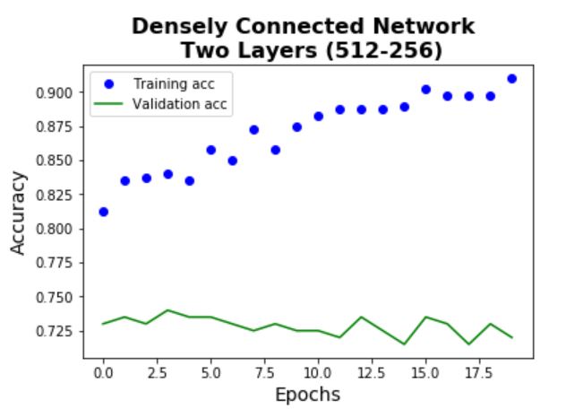
Model 1 - Baseline Model

Before building CNN models, a baseline densely connected network model is built. This step is important as the final CNN model can only be accepted if it can beat the performance of the cheaper and simpler alternative models. Notice that there is significant overfitting for this model. The test performance gives an accuray of 74%.

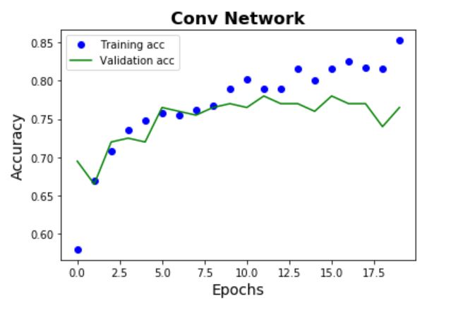
Model 2

Compared to the baseline model which contains 2 dense layers, the first CNN model adds 3 Conv layers and Pooling layers on top of the 2 dense layers. From the plots below, it can be seen that the validation performance is slightly better than the baseline model, and there is much less characteristics of overfitting. An accuracy of 78% is given by the test set.

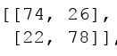
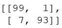
Error analysis

It is also important to look at how well the model performs on classifying each class (for this problem it is inappropriate to use recall/precision as the performance metric since no class is more important than the other). From the confusion matrix below, it can be seen that the model has roughly the same performance for both classes. Class 0 - Mountain and Class 1 - Sea.

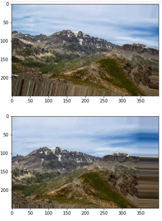
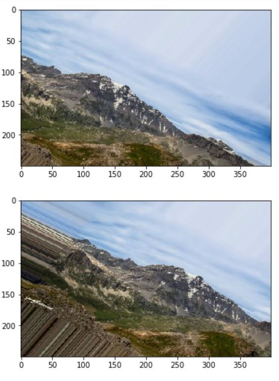
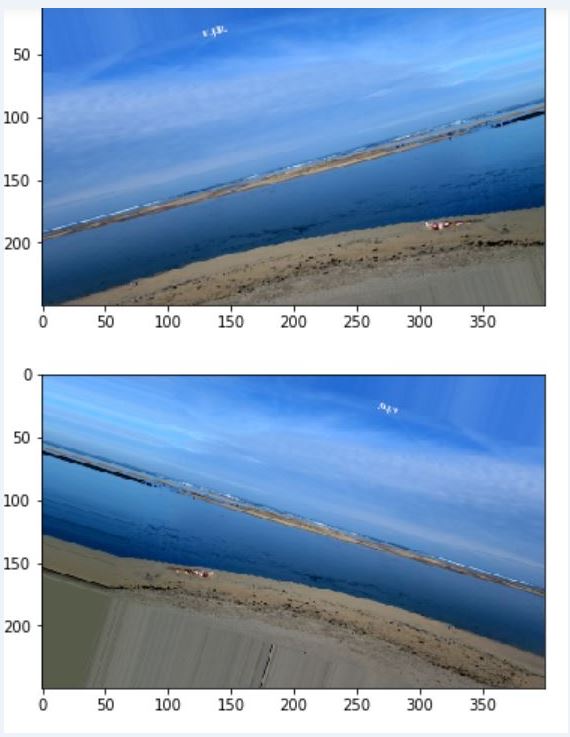
Model 3 - Use Data Argumentation

The best way to reduce overfitting and improve the generalization power of the model is to collect more training samples, however, in this case it is not possible to get more photos and one way to substitute this is to ARGUMENT the photos through some sort of transformations on the training images - this can include rotation, translation, zooming, adding noisy, etc. Examples of argumented images are shown below.

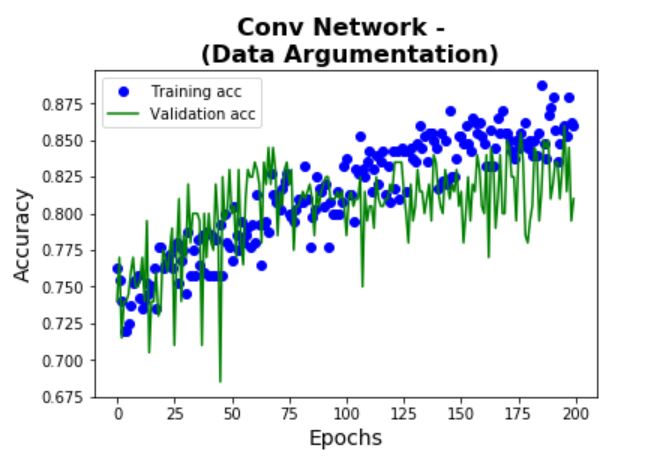
To see the impact of data argumentation, Model 3 has the same architecture as Model 2. From the plots below, it can be seen that the validation performance is MUCH better than that of Model 2, and there is MUCH less characteristics of overfitting. An accuracy of 88% is given by the test set (10% improvement than Model 2).

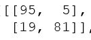
Error analysis

From the confusion matrix below, it can be seen that the model has better ability to classify correctly a mountain picture than a sea picture (i.e. sea pictures are more likely to be considered as mountain pictures by the model) - one possible explanation can be that the argumentation methods applied are better choices for mountain images than for sea images.

Model 4 & 5 - Using Pre-trainined Model (Feature extraction)

One popular approach to improve the predictive power on small image dataset is to use some pre-trained neural networks (usually the popular ones that were built for large datasets). For this problem, the pre-trained VGG16 is downloaded. The idea is to use the representations learned by the pre-trained model (which already learned much of the spatial hierarchy of features in some images) to extract features from the training samples. Note that only the convolutional layers (convolutional base) will be used to extract the features - we want to make the final model specific to the current problem.

Note that two different models are built:

1. Model 4: Without data argumentation (cheaper): running the convolutional base over the training samples, and then use the extracted features as input into the dense layers.
   
2. Model 5: With data argumentation (more expensive): first add the dense layers on top of the convolutional base, and then running the whole model over the training samples.

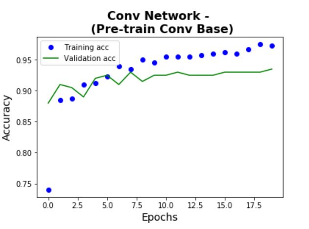
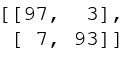
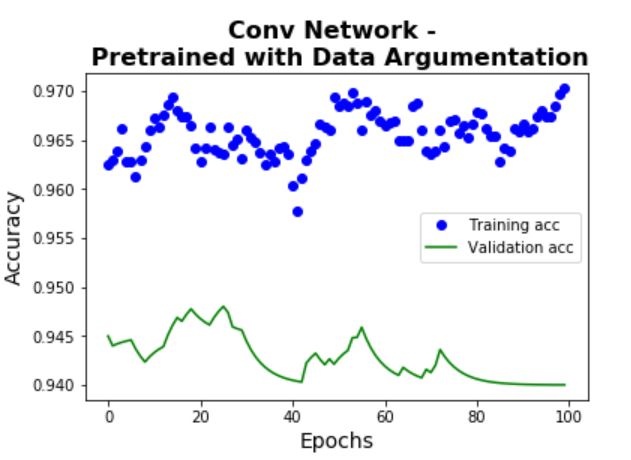
The learning curves and confusion matrix on the test set are shown below. Using the test set, Model 4 achieves an accuracy of 95% and Model 5 achieves an accuracy of 95.5% (significant improvement from Model 3). In addition, the amount of overfitting is also quite small given the high accuracy. This shows the power of using pre-trained models.

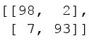
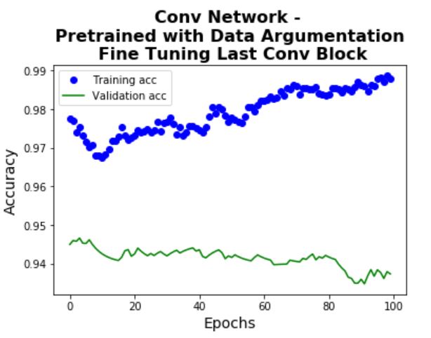
Model 6 - Using Pre-trainined Model (Fine tuning the top layers)

Model 6 uses another approach commonly applied with pre-trained models - jointly training both the top layers and the dense layers. The idea is that top layers are learning the more abstract representations and re-train these layers could possibly make them more powerful for the current problem. In this case, only the top convolutional block is tuned (where in other cases could re-train the top few layers/ blocks). Results are shown below. Note that an accuracy of 96% is achieved on the test set (a very slight improvement compared to Model 4 & 5).

Visualize & Interpret the ConvNets

Compared to other deep learning models, CNNs are not purely black boxes - in the sense that it is possible to understand (at least partially) how a ConvNet is learning the representations.

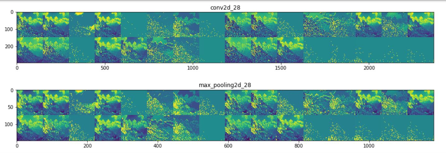
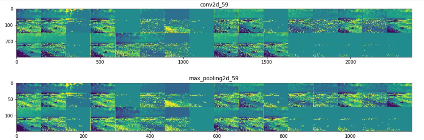
1. Intermediate Activations

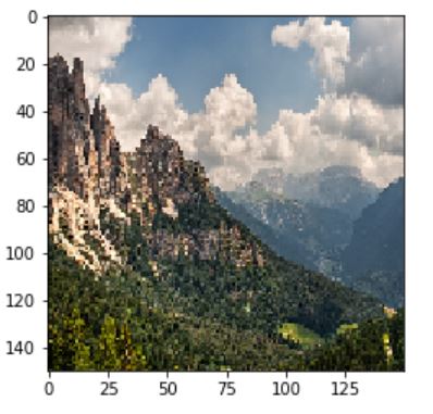
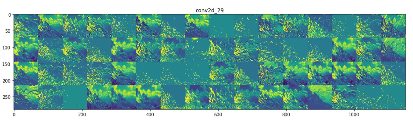
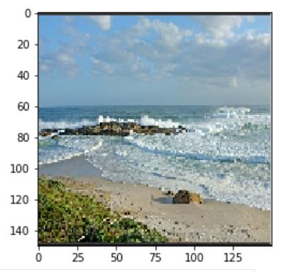
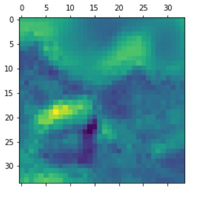
This method visualizes what the activations look like from each filter of each convolutional layer. Note that for this method one has to perform the exercise for many images (as for each image the intermediate activations will be different), however, it is possible to identify some patterns on how the activations look like using multiple images. Below shows the intermediate activations (from the three convolutional layers) for an mountain image (using Model 3). It can be seen that higher layers are more like the original picture where the deeper layers are very abstract (possibly capturing the details).

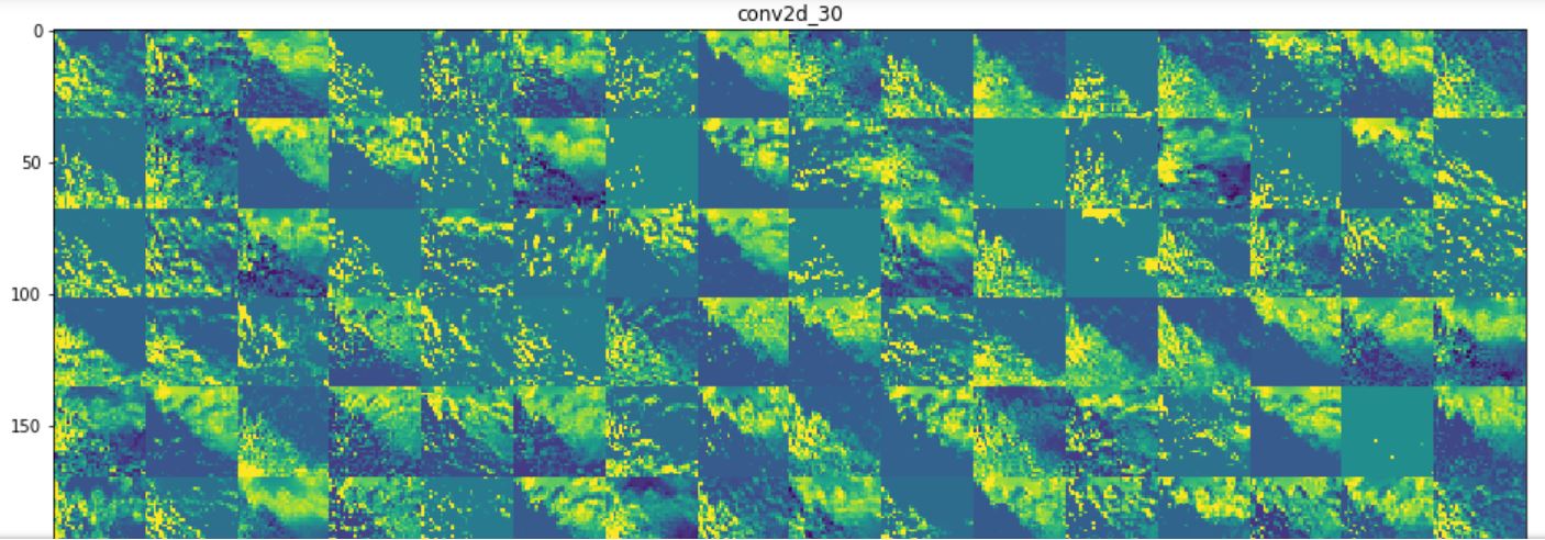
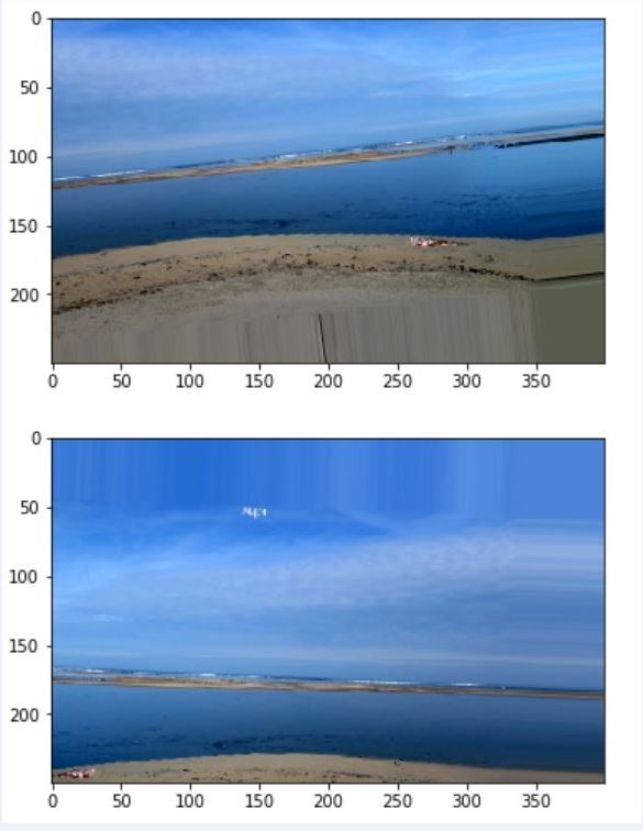
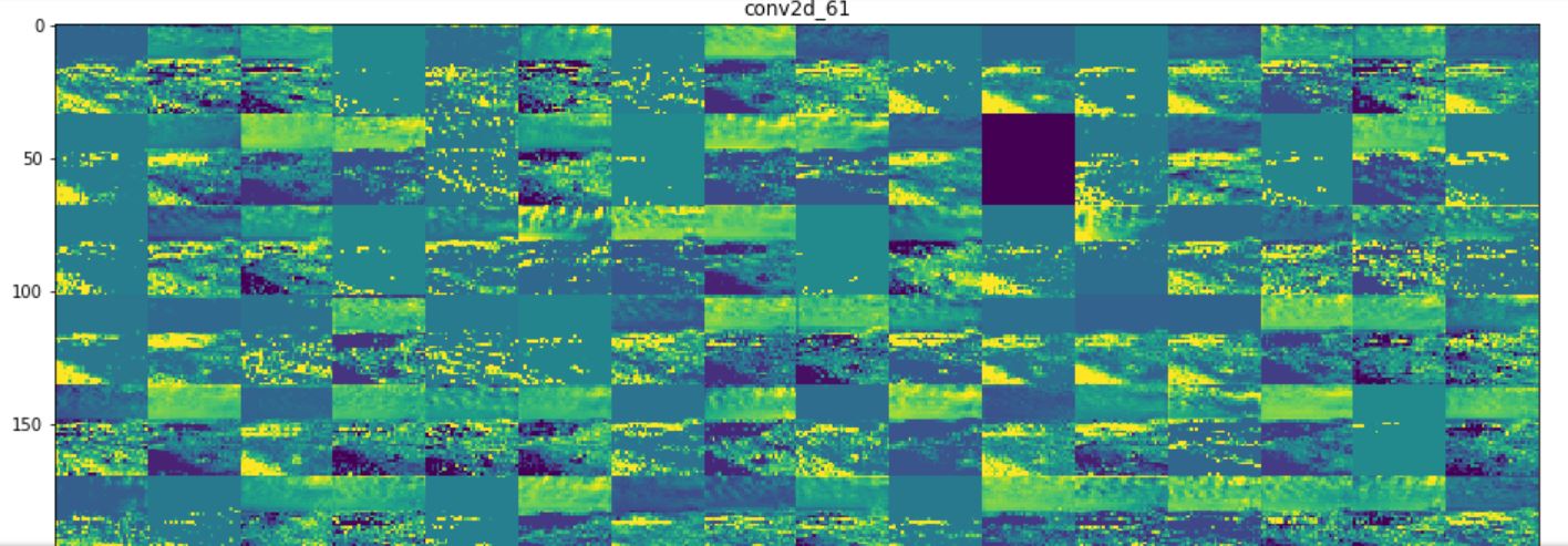
Now the activations for a sea image. Note that the deeper layer (third image) has a black filter - means that filter is learning nothing about the image (this possibly explains why the model is better at recognizing mountains than seas - the filters possibly are more powerful for mountain pictures).

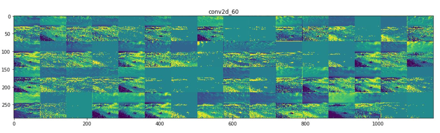
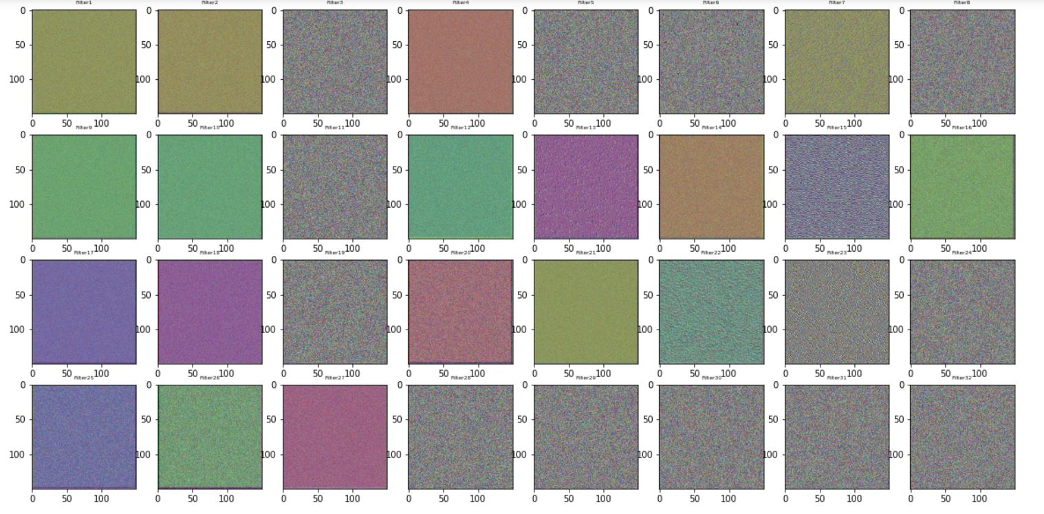
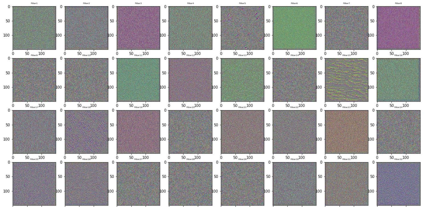
2. Filters

For this method one does not need to perform it over different images, as it allows us to see what each filter in each layer is encoding by displaying the pattern that each filter is encoding. The way to do this is simple - use GRADIENT ASCENT to maximize the response of the filter (loss function that maximizes the filter, then use gradient descent to optimize the input to maximize the activations). The patterns encoded by the first 32 filters in convolutional layer 1 & 2 in Model 3 are displayed as follows. Again it can be noticed that deeper layer (layer 2) is capturing more detailed information (e.g. the wave-like texture/linetype and more complex colour patterns).

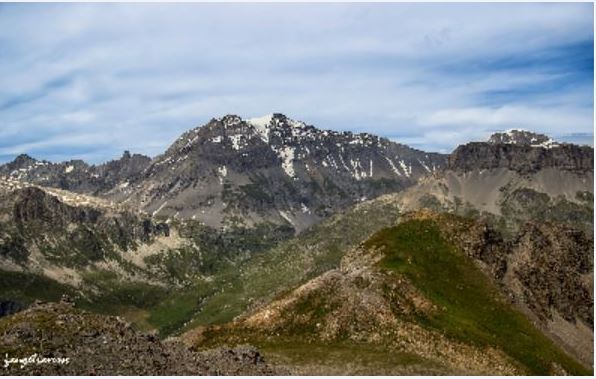
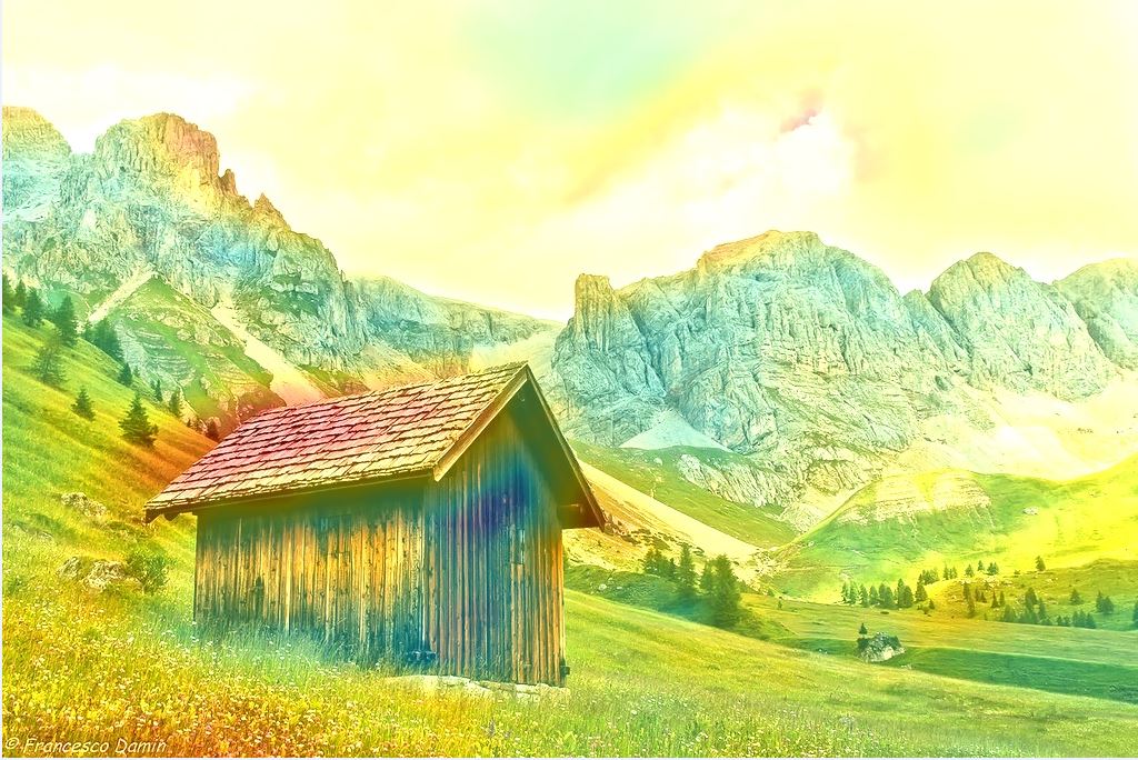
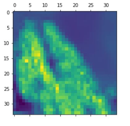
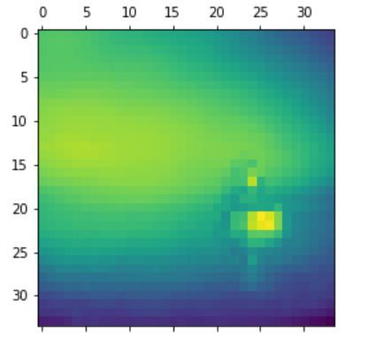
3. Class Activation Map (CAM)

Like method 1 for this method we need to perform it for each image, but it is quite powerful as it tells us for the given image why did the model think the image is mountain/sea by locating the most important areas in the image. In this case, it builds a heatmap of scores using GRADIENT-BASED LOCALIZATION - weighting input activates different channels and weighting each channel with respect to each class. 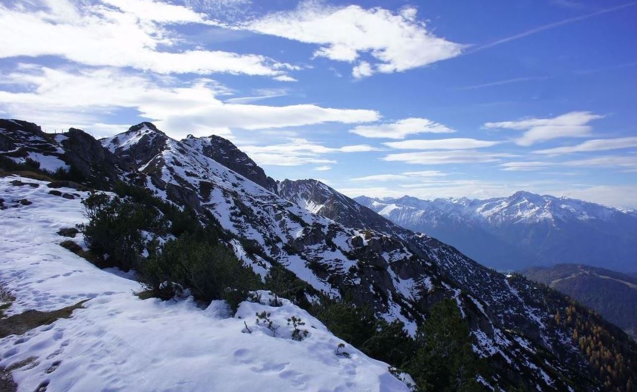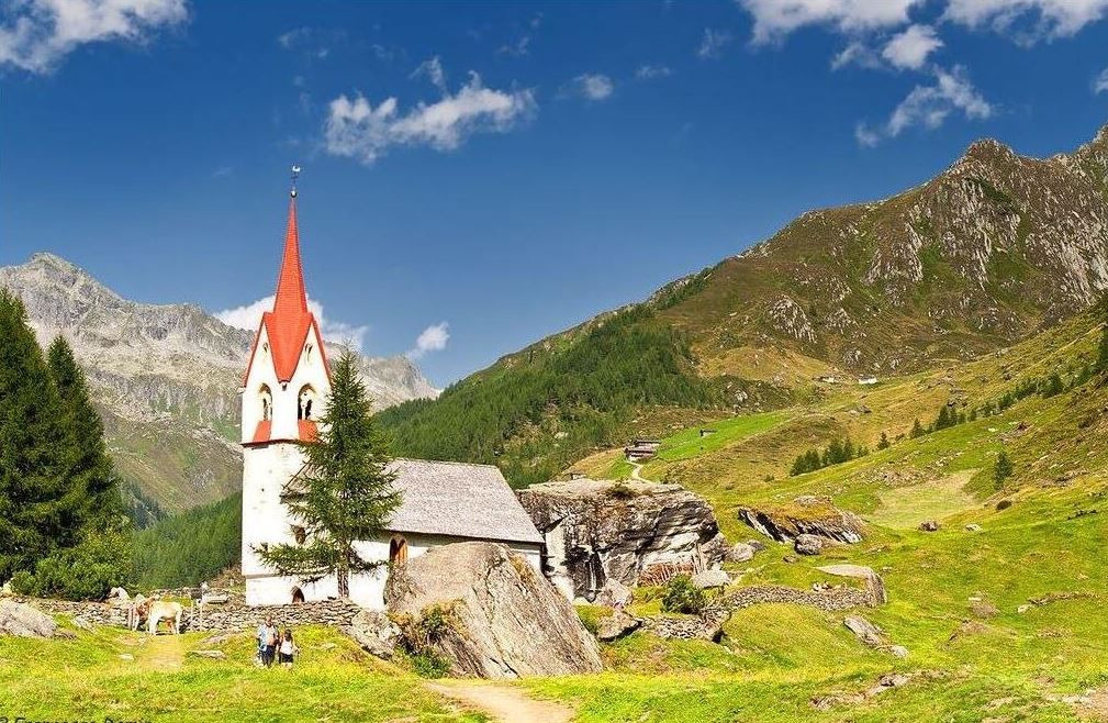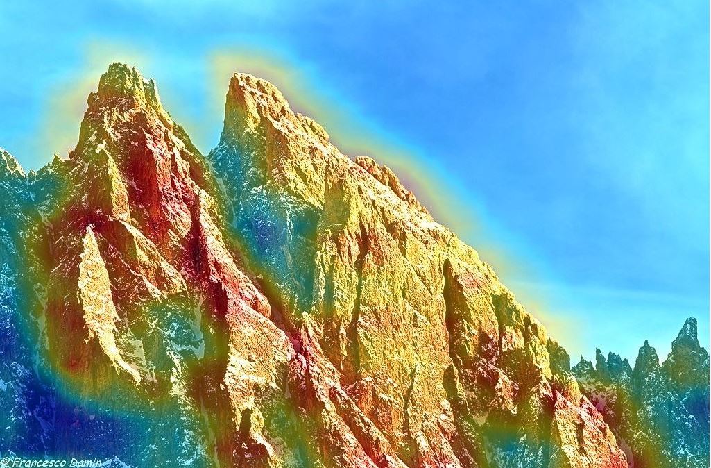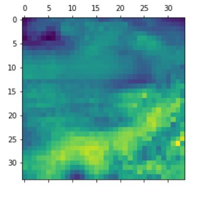The following is an example of the heatmap overlaying on top of two mountain images. It can be seen that in the second image, the model almost perfectly identifies the mountain in the picture (brighter colours) where in the first image, the model captures both the mountain at the background as well as the small house at the front.

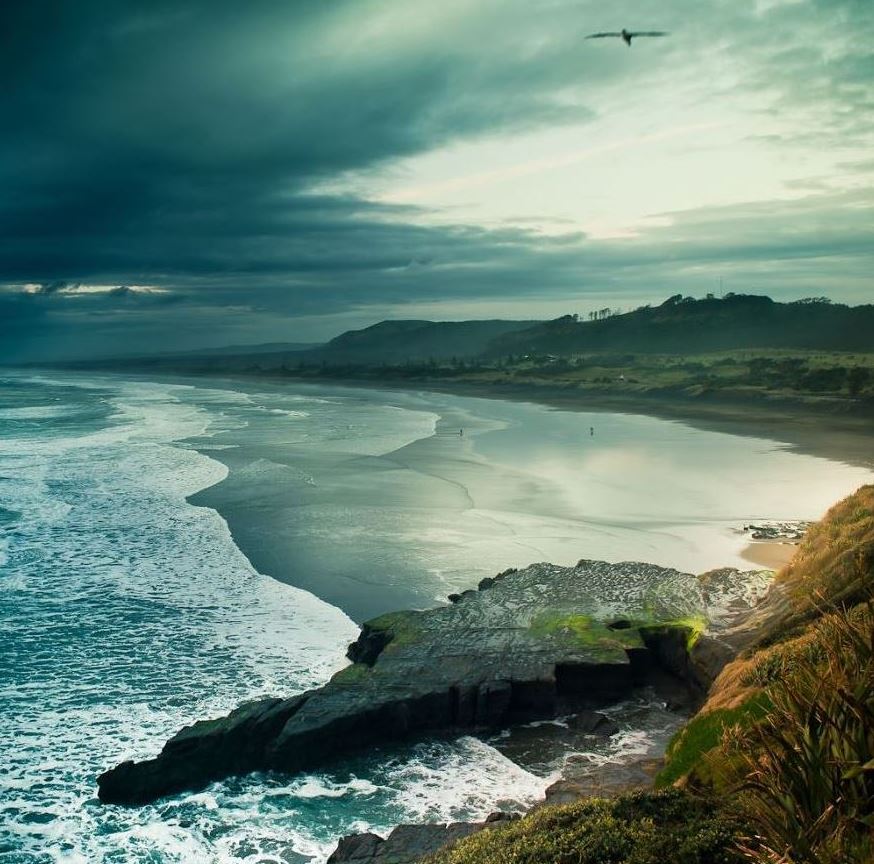
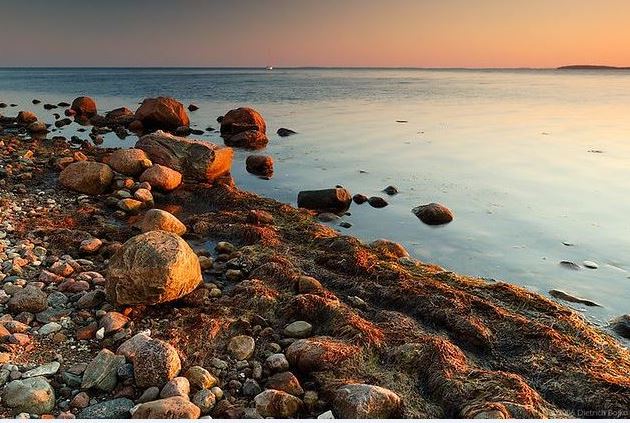
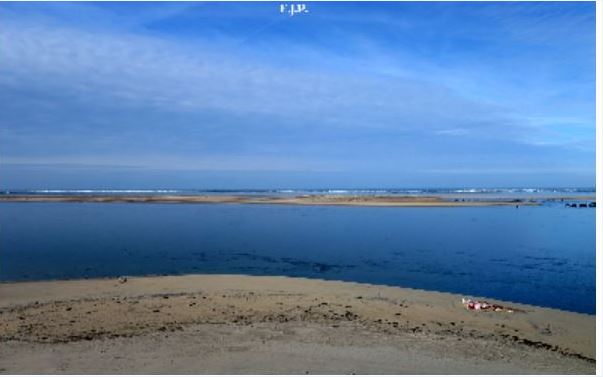
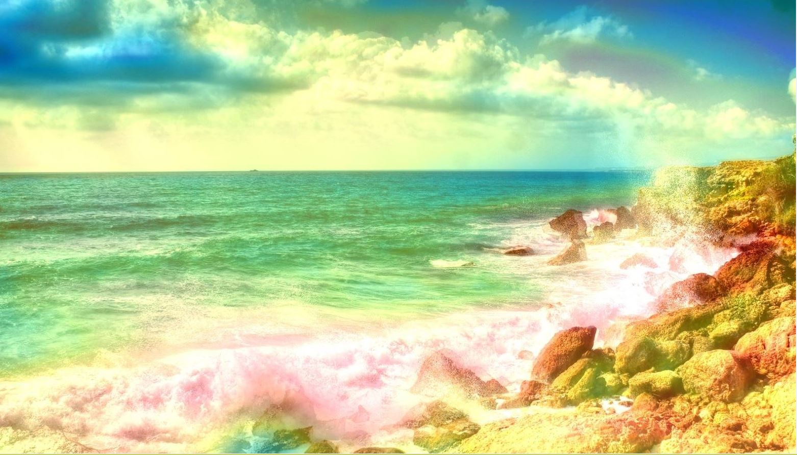
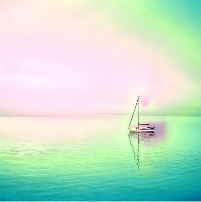
Now look at 2 sea images. It can be seen that in the first image, the model identifies image as a sea because it captures the big wave close to the beach. For the second image, the model thinks it is a sea as it captures not only the sky (touching with the sea) but also the small boat in the picture.

Remarks

In case where the model is not performing well, this method allows us to see why the model fails to correctly classify some images and can let us understand which features are the model is not learning well. As a result, one way to improve the performance is to obtain more images that focus more on these features to help the model better learn. Therefore, visualizing ConvNets can be useful tools for error analysis.

Last updated on Jan 1, 2020