Bayesian inference for exponential distribution model using relative belief

In general, how to measure statistical evidence precisely in Bayesian analysis is a challenging problem. This project discusses how to make inference for the exponential distribution model in the context of Bayesian analysis, using a particular measure of evidence – the relative belief ratio, to illustrate how it can be used to make statistical reasoning precisely.

Throughout the project, the evidential approach to the proposed statistical problem is emphasized, and analyses include the following sections

prior elicitation
control of biases of model and prior
model checking
prior-data conflict

to make sure the final inferences (estimation and hypothesis assessments) made are accurate and meaningful.

Bayes factor vs Relative belief ratio

Bayes factor

Within the Bayesian inference context, one popular method to measure statistical evidence is to use the Bayes factors, where large values of Bayes factors correspond to strong evidence for hypothesis assessments. However, it has been shown that in some examples such as the Jeffreys-Lindley’s paradox, the Bayes factors can be problematic and cannot fit into the general theory of statistical reasoning (strictly speaking).

Jeffreys-Lindley’s paradox:

If one makes the prior more diffuse then there will be more supports for the hypothesis based on measures such as Bayes factors. In this case, although making prior more diffuse seems to make the prior more uninformative, it is actually creating more bias in favor of the hypothesis and therefore making the inference unreliable. Wiki's page on the Jeffreys-Lindley’s paradox

Relative belief ratio

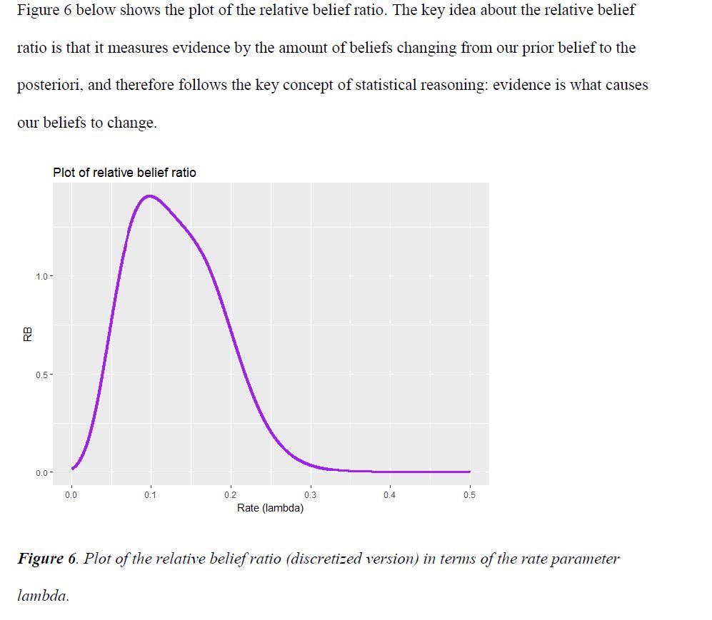
As opposed to measures such as Bayes factors, for the relative belief principle, measure of evidence is separated from the measure of its strength, and therefore can solve many of the paradoxes. In other words, the relative belief ratio seeks to measure evidence by the amount of belief change from priori to posteriori, and uses probability to only measure the strength of evidence but not the evidence itself.

Elicitation procedure for the prior

The first step is to select a prior for the rate parameter (lambda) of the exponential distribution model. For this problem, the prior distribution π(.) is selected to be the gamma distribution for the following reasons:

Gamma distribution has support over (0,∞) as the rate parameter 𝜆 needs to be strictly positive
Gamma distribution can take very flexible shapes (therefore we can make the prior less informative if needed)
The conjugate prior for the exponential distribution is the gamma distribution (unless there is a strong reason to reject the gamma family, using a conjugate prior is convenient)

The prior is then estimated numerically using the data.

Control of bias due to model and prior choices

The second step involves how to quantify both the bias against and bias in favor for hypothesis assessments in this problem. This gives a way to see if the selected prior is inducing significant bias into the inference, and therefore to decide whether another prior should be used.

Derive the prior predictive distribution. Here, instead of deriving the prior predictive distribution in terms of the original random variable, the minimal sufficient statistic T(X) is being used as we want the analysis only depends on the data through the minimal sufficient statistic.
Bias against the hypothesis assessment. Using the principle of evidence, the bias against of H0: λ= λ0 is is the prior probability measure of the data given the null hypothesis is true.
Bias in favor of the hypothesis assessment. Bias in favor occurs when evidence against is not obtained when the null hypothesis is false with high prior probability.

Model checking based on the observed data

The third step is to estimate the model based on the data. The following procedures are involved in this step:

Numerical assessment (one-sample Kolmogorov-Smirnov test)
Graphical assessment (kernel density plot)

Checking for prior-data conflict based on the observed data

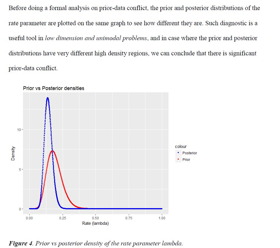
After making sure the sampling model is a reasonable choice for the observed data, now it is important to make sure the selected prior does not have significant conflict against the observed data. Prior-data conflict essentially means that the selected prior is placing most of its mass on parameter values which is surprising given the observed data.

Diagnostics - Where the prior and posterior distributions have very different high density regions, we can conclude that there is significant prior-data conflict.
Using the prior predictive distribution - Formal measure which involves the prior predictive distribution with the minimal sufficient statistic (tail probability is computed).

Inferences based on relative belief

Estimation
Hypothesis Testing

Last updated on Nov 1, 2019